
Update automatically a trend chart using name manager in an excel report
In the IT service management, it is normal to use a trend chart to show the result of the last 12 months to see in a quick way the evolution. In fact, the trend chart is not only used in IT, other departments like finance are also using it. If I have only 1 chart, it is not really a big deal but when I have 10 or more, if I have to do it manually, I am not really optimizing my time so not really a time saving. In excel, there is an option so each time I put the new value, the trend chart will be updated automatically.
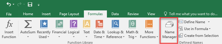
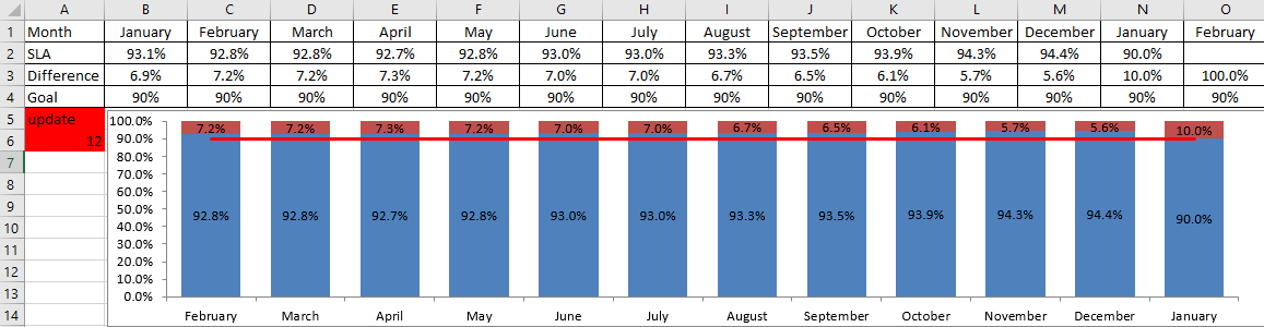
This option is called “name manager”. Unfortunately, it is not just clicking in this option and all done, a little work has to be done first. For a good explanation, I will take 2 examples, a vertical one that I will call VER in the VLSA sheet and an horizontal calling HOR in the HSLA sheet.
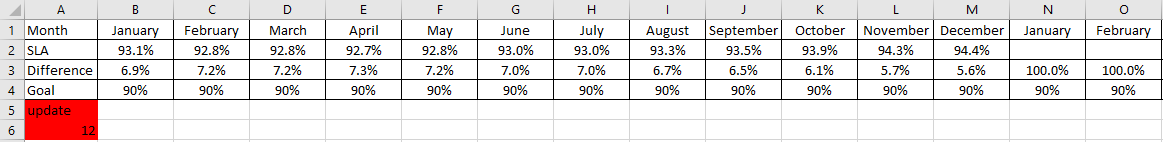
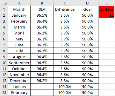
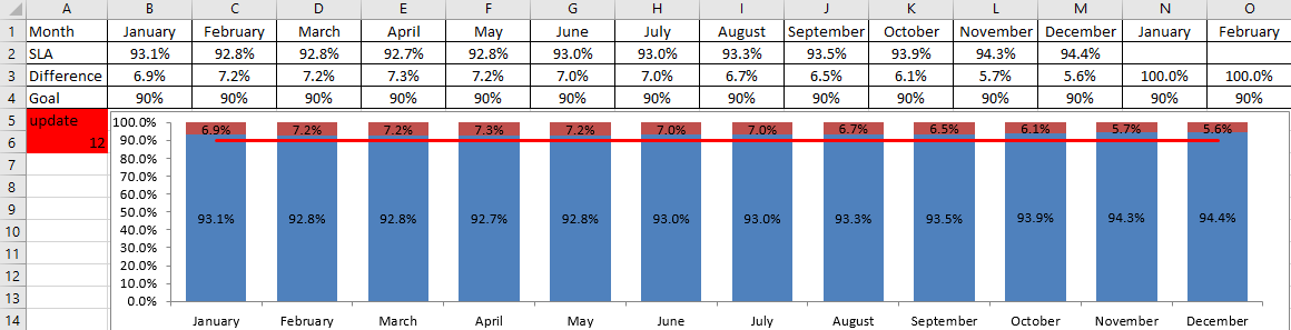
1. Defining the number of months to update. You have to put in a cell the number of months you want to update your chart. For instance, put 12 if you want to update the last 12 months, 6 for the last 6 months, 15 for the last 15 months, etc. And most importantly, it should be in a cell out of the value range. For instance, for VSLA is on A6 and for the HSLA on E2.
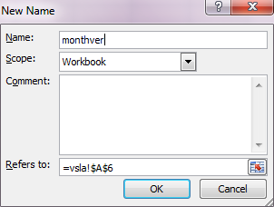
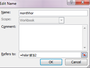
2. Referring the number of months to update. For VLSA, select this cell and once you click on the “name manager” function, click “new” and in name put “monthver” then click “OK”. Do the same for HSLA but put the name “monthhor”.
 |
 |
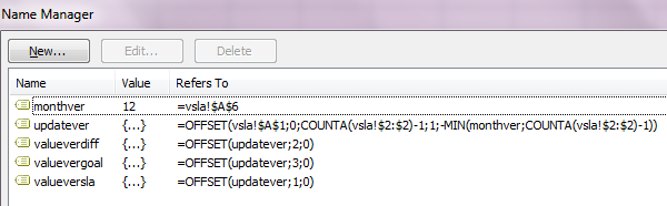
3. Defining how to update the chart automatically. This is the trickiest part because it is here that you will define how you want your chart to be updated automatically. Click to “new” again and for VSLA put the name “updatever” and in “refers to”, put:
- =OFFSET(vsla!$A$1;0;COUNTA(vsla!$2:$2)-1;1;-MIN(monthver;COUNTA(vsla!$2:$2)-1))
- Explanation:
- $A$1 is referring to the first cell of the month range. It should not be empty, I put “month” but you can put date, report, etc.
- $2:$2 is referring to the row2, in this case the SLA one. I am telling it to update the chart when I put a new value in this range. If you want for instance that each time you put a new value for the row3 (the “difference” one), change it to $3:$3
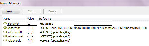
For HSLA, put the name “updatehor” and in “refers to”, put:
- =OFFSET(hsla!$A$1;COUNTA(hsla!$B:$B)-1;0;-MIN(monthhor;COUNTA(hsla!$B:$B)-1);1)
- Explanation:
- $A$1 is referring to the first cell of the month range. Also, it should not be empty.
- $B:$B is referring to the column B, in this case the SLA one. If you want for instance that each time you put a new value for the column A (the “month” one), change it to $A:$A
4. Referring the “SLA” range. Click again to “new” and for VSLA, in name put “valueversla” and in “refers to”:
- =OFFSET(updatever;1;0)
- Explanation: 1 is the first row below the month row.
For HSLA, in name put “valuehorsla” and in “refers to”:
- =OFFSET(updatehor;0;1)
- Explanation: 1 is the first column after the month column.
5. Referring the “difference” range. Do the same thing as for the step 4, just put another name and instead of 1, put 2. For instance, =OFFSET(updatever;2;0) for VSLA and =OFFSET(updatehor;0;2) for HSLA
6. Referring the “goal” range. Do the same thing again by putting a new name and instead of 1, put 3
 |
 |

So now we have everything configured but we still have one last thing to do, we need to link them to our chart so select your chart or create it and go to “select data”. I will explain only for the VSLA sheet because it will be the same for HSLA:
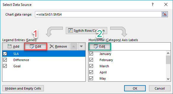
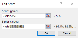
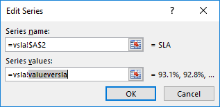
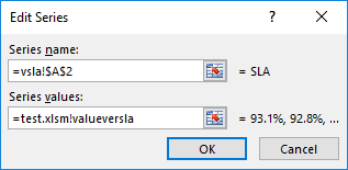
- 1. On the left side, select “SLA” and click on “edit”. In “series values”, change “$B$2:$M$2” by “valueversla” then click “OK”.
 |
 |
 |
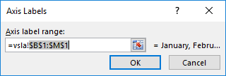
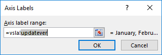
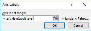
- 2. On the right side, click on “edit” In “axis label range”, change “$B$1:$M$1” by “updatever” then click “OK”.
 |
 |
 |
- 3. Do the same thing for “difference”, for the right side, it is “valueverdiff” and right side, it is “updatever”
- 4. Do the same thing for “goal”, for the right side, it is “valuevergoal” and right side, it is “updatever”
- 5. Once all done, just click to “OK”.
Now your chart will be updated automatically each time you put a new value in the SLA range, for instance, if you put a value on cell N2, you will see it.As I said, for HSLA, it is the same process. The only difference is the name, for instance for SLA, for the left side, it is “valuehorsla” and the right side is “updatehor”.
Interesting Management
-

Part 1: A good manager, better team motivation, better team productivity, better team results
When you are managing a team, “how to be a good manager” is the “must”...
-

Report optimization, increase your time management
As manager, I am doing many reports, even when I was an ITIL consultant, I still needed to do many reports...
-

Tools to get your ITIL intermediate certifications, the missing 15 points for the ITIL 4 Managing Professional
ITIL V3 is going to be obsolete...
-

The importance of the first customer meeting for the service
Managing an IT service when I start a new company is not an easy task, particularly true, if the service...
-

1 click macro tool: Incident/Problem Management - create a daily report in excel
This file will allow you to have in one single excel file the issues (incidents, problems, outages, major incidents...
-
1 click macro tool: Incident/Problem Management - create a daily report and a public version in excel
This file is an extended version of the above that includes the option to create a public version to share with...
-
1 click macro tool: Problem/Incident Management - compile multiple daily excel files in 1 with access
This file will allow you to compile all daily issues reported in excel in 1 single excel file in xlsx format...
-
1 click macro tool: Incident/Problem Management - create a monthly report in excel
This file will allow you to create a monthly report related to daily issues and updating all pivots, charts and...
-
1 click macro tool: Problem/Incident Management - create daily reports and compile them in 1 to create the monthly report in excel
This tool will create daily reports then compile them to create the monthly...
-

Calculate a weighted average for a SLA and a conversation time with a formula in an excel report
In one of my experiences, I had a tool that gave me the weighted average...
-
Search in different sheets then display the wanted data with a formula in an excel report
vlookup and hlookup are formulas that allow to search a data in another...
-
Find the good data by matching 3 different criterias with a formula in an excel report
It is a combination of “index” and “match” formulas, much better...
-
Sum and count sales with a formula in an excel report
Extracting data from salesforce or qlikview may not give the information I needed, it already happened...
-
Know how long a service is impacted with a formula in an excel report
It is important to know how long the service has been impacted by...