For one of my reports, I had the challenge to find a way to display all main ID (because some are missing) by looking into the sub-ID based on 2 extracted reports, 1 containing the main ID and 1 containing the sub-ID. The point was that the ticketing system didn’t allow to have all the data in one single file and also, putting the same period of time, the result was not the same, apart the ID, one listed less information than the other.

It is not easy to explain but may be with an example. The main task ID report showed different information than the sub task ID report, only the configuration item is the same for both. The main task ID can have many sub task ID and of course, the numbers are different. This is the reason why one listed more information than the other. To resume, I had to create a circling formula (not a looping formula) to find the missing main ID.

 

When I use the formula ?

I used a report that I had all the information needed but in case if this report didn’t work, I needed to use another system to extract the data manually so as a workaround.

 

How to use the formula ?

The formula in this topic is with "," so depending of the operating system of your PC, the formula should have ";" instead of ",".

 

How are the formulas ?

=IF()

=IFERROR()

=VLOOKUP()

The formulas are very simple, the difficult part is the order and if it was worth to do it in 1 or 2 formulas. As you can see below, I opted for 2 formulas (column E and F) because when I tested in 1 formula, it was creating a looping that didn’t work out properly so I needed to divide it.

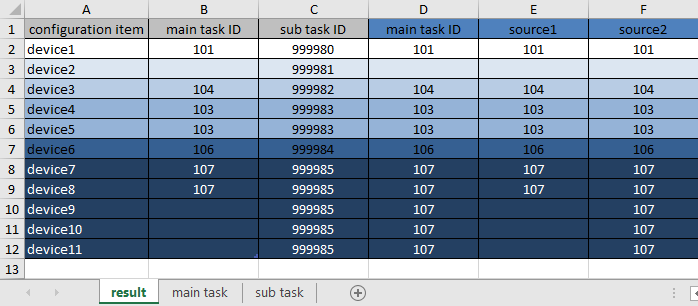
• For the column A in cell A2:
  =IF('sub task'!A2=0,"",'sub task'!A2)
  It will list all devices of the sub-task sheet in column A because, as I said, a main task can have many sub tasks
• For the column B in cell B2:
  =IFERROR(VLOOKUP(A2,'main task'!A:H,3,0),"")
  It will show the ID of the main task sheet of column C (3 = C) if the name of device matches in the column A ofthe main task sheet
• For the column C in cell C2:
  =IFERROR(VLOOKUP(A2,'sub task'!A:F,2,0),"")
  It will show the ID of the sub task sheet of column B (2 = B) if the name of device matches in the column A ofthe sub task sheet
• For the column D in cell D2:
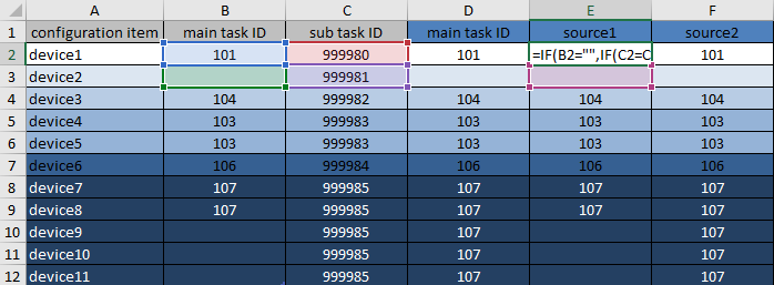
  =F2
• For the column E in cell E2:

=IF(B2="",IF(C2=C3,IF(B3="",IF(C2=C3,IF(E3>1,E3,""),""),B3),""),B2)

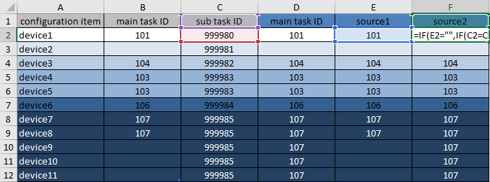
• For the column F in cell F2:

=IF(E2="",IF(C2=C1,IF(F1>1,F1,""),""),E2)

If you don’t know how to use the vlookup, read Search in different sheets then display the wanted data with a formula in an excel report.

My goal was to find all main task ID for the column B based on the sub task ID. As you can see, in the column D, I have the information except for the cell D3, this is because the configuration item “device2” didn’t exist in the “main task” sheet. I highlighted by color so it is easier to see which one is single and which one not.