

Formula: sum weekend values to show only week date in an excel report
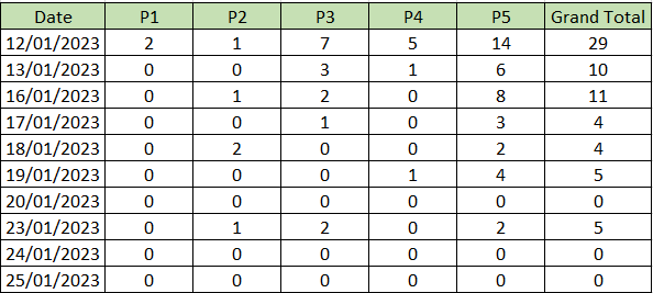
I have this table with some dates that fall in the weekend (Saturday and Sunday):
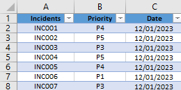
I want to calculate how many incidents I have but for my final results, I don’t want to show those weekends. I want to sum values of the weekend into the next week day, in this case, on Monday. If you are looking for the Power BI version, read Power BI: sum weekend values to show only week date.
When I use the formula ?
To calculate all values without showing the weekend.
How to use the formula ?
The formula in this topic is with "," so depending of the operating system of your PC, the formula should have ";" instead of ",".
How are the formula ?
=IF()
=OR()
=TEXT()
=IFNA()
=VLOOKUP()
=IFERROR()
=GETPIVOTDATA()
=SUM()
=COUNTIFS()
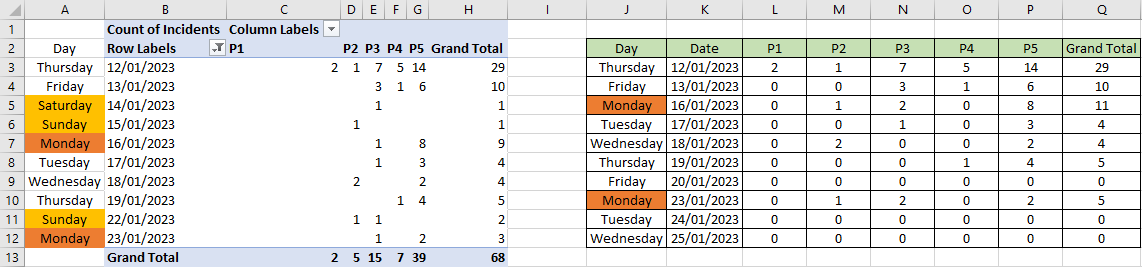
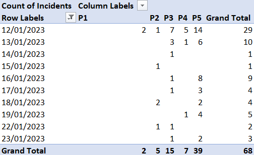
First thing it is to create a pivottable, it is much easier (later I will show how to do it without it):
I will create a calendar without weekend by putting in the cell K3, this simple formula making reference to the first day of my column “date”:
=B3
In the cell K4, I will put this formula:
=K3+IF(OR(TEXT(K3+1,"ddd")="sat",TEXT(K3+1,"ddd")="sun"),3,1)
And just copy it to below cells.
In the cell L3, I will make reference to the result of P1 in the pivotable, in fact, I just want excel to give me the formula, which is:
GETPIVOTDATA("Incidents",$B$1,"Priority","P1","Date",DATE(2023,1,12))
I will change the last part “DATE(2023,1,12)” by “$K3”:
GETPIVOTDATA("Incidents",$B$1,"Priority","P1","Date",$K3)
And with that, I will create my final formula so in my cell L3, it will be:
=IF(IFNA(VLOOKUP($K3,$B:$B,1,0),0),IF(TEXT($K3,"ddd")="mon",IFERROR(GETPIVOTDATA("Incidents",$B$1,
"Priority","P1","Date",$K3),0)+IFERROR(GETPIVOTDATA("Incidents",$B$1,"Priority","P1","Date",$K3-2),
0)+IFERROR(GETPIVOTDATA("Incidents",$B$1,"Priority","P1","Date",$K3-1),0),IFERROR(GETPIVOTDATA
("Incidents",$B$1,"Priority","P1","Date",$K3),0)),0)
I will copy this formula to the rows below and to the columns beside without forgetting to change P1 by P2, P3, P4 and P5. For the last column “Grand total”, I can use the same process:
=IF(IFNA(VLOOKUP($K3,$B:$B,1,0),0),IF(TEXT($K3,"ddd")="mon",IFERROR(GETPIVOTDATA("Incidents",$B$1,
"Date",$K3),0)+IFERROR(GETPIVOTDATA("Incidents",$B$1,"Date",$K3-2),0)+IFERROR(GETPIVOTDATA
("Incidents",$B$1,"Date",$K3-1),0),IFERROR(GETPIVOTDATA("Incidents",$B$1,"Date",$K3),0)),0)
NOTE: the formula is shorter because it doesn’t include the “priority” (P1, P2, etc.)
Or just do a SUM formula like that for the cell Q3:
=SUM(L3:P3)
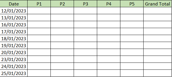
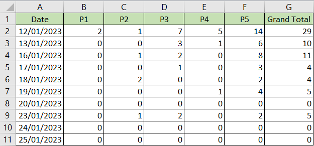
Now if I don’t want to use a pivot table, I can get the same result with one table. For that, I will create the calendar without weekend by putting in the cell A2 the first date which is the 12/01/2023 and in the cell A3, the same formula as the one above:
=A2+IF(OR(TEXT(A2+1,"ddd")="sat",TEXT(A2+1,"ddd")="sun"),3,1)
NOTE: don’t forget to change the cell reference
From this point, the formula will be different. So in the cell B2, put this formula:
=IF(IFNA(VLOOKUP($A2,Sheet1!$C:$C,1,0),0),IF(TEXT($A2,"ddd")="mon",SUM(COUNTIFS(Sheet1!$B:$B,"P1",
Sheet1!$C:$C,$A2))+SUM(COUNTIFS(Sheet1!$B:$B,"P1",Sheet1!$C:$C,$A2-2))+SUM(COUNTIFS(Sheet1!$B:$B,
"P1",Sheet1!$C:$C,$A2-1)),SUM(COUNTIFS(Sheet1!$B:$B,"P1",Sheet1!$C:$C,$A2))),0)
Copy it rows below and also in the next columns, just don’t forget to change P1 by P2, P3, etc. And for the last column, I just do a SUM.
Interesting Management
-

Part 1: A good manager, better team motivation, better team productivity, better team results
When you are managing a team, “how to be a good manager” is the “must”...
-

Report optimization, increase your time management
As manager, I am doing many reports, even when I was an ITIL consultant, I still needed to do many reports...
-

Tools to get your ITIL intermediate certifications, the missing 15 points for the ITIL 4 Managing Professional
ITIL V3 is going to be obsolete...
-

The importance of the first customer meeting for the service
Managing an IT service when I start a new company is not an easy task, particularly true, if the service...
-

1 click macro tool: Incident/Problem Management - create a daily report in excel
This file will allow you to have in one single excel file the issues (incidents, problems, outages, major incidents...
-
1 click macro tool: Incident/Problem Management - create a daily report and a public version in excel
This file is an extended version of the above that includes the option to create a public version to share with...
-
1 click macro tool: Problem/Incident Management - compile multiple daily excel files in 1 with access
This file will allow you to compile all daily issues reported in excel in 1 single excel file in xlsx format...
-
1 click macro tool: Incident/Problem Management - create a monthly report in excel
This file will allow you to create a monthly report related to daily issues and updating all pivots, charts and...
-
1 click macro tool: Problem/Incident Management - create daily reports and compile them in 1 to create the monthly report in excel
This tool will create daily reports then compile them to create the monthly...
-

Calculate a weighted average for a SLA and a conversation time with a formula in an excel report
In one of my experiences, I had a tool that gave me the weighted average...
-
Search in different sheets then display the wanted data with a formula in an excel report
vlookup and hlookup are formulas that allow to search a data in another...
-
Find the good data by matching 3 different criterias with a formula in an excel report
It is a combination of “index” and “match” formulas, much better...
-
Sum and count sales with a formula in an excel report
Extracting data from salesforce or qlikview may not give the information I needed, it already happened...
-
Know how long a service is impacted with a formula in an excel report
It is important to know how long the service has been impacted by...