

Power BI: convert decimal to unique number for filter
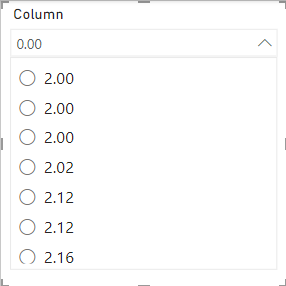
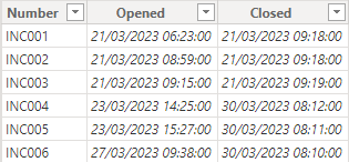
When I work with date and/or time, I can’t use decimal numbers as a vertical list, tile or dropdown slicer because usually there will be duplicate. For instance (left picture):
| single selection dropdown filter | between filter |
 |
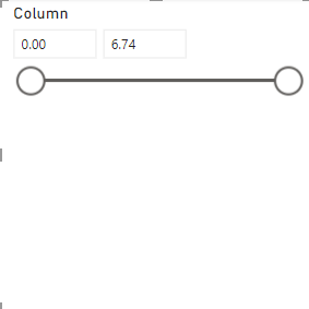 |
Of course, I can use the between filter (right picture) but based on the type of report, sometimes, I prefer to use the others. In fact, there is no issue at all using it like that but seeing multiple times same values, it is quite confusing. In my example, to select the value 2.00, it appears 3 times and I need it only 1.
Converting the column as whole number it is not a solution because it will round up or down the number. For instance, values between 2.5 and 3.5 will be 3 but if I select 3 in my slicer, I don’t want to show in my table or to calculate in my visual card everything above 3. At the end, in my mind, selecting 3 means “3 and below” and not “3 and above”. Neither using functions like ROUND, DATEDIFF, etc. will resolve it.
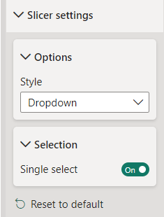
The solution I found it is to use the TRUNC function. It will extract the digits before the dot, for instance 241.56 will be 241. Here is my logic, as you can see in the picture above on the left, my filter is a dropdown one with a single selection (left picture). I need to convert it into single unique value like that (right picture):
 |
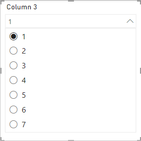 |
So when I select a number, I want to show everything equal and below meaning “2 and below” and nothing above it meaning 2.01, 2.02, etc. For that, I need to tell Power BI:
- 1. Every integer number should stay as it is. For instance, 1 = 1, 7 = 7, etc.
- 2. Every value above the integer but below the upper one should be considered as integer number. For instance 1.01 = 2, 1.47 = 2, etc.
So the result will be:
- 0.00 = 0
- 0.01 -> 0.99 = 1
- 1.00 = 1
- 1.01 -> 1.99 = 2
- 2.00 = 2
- Etc.
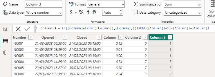
This is my formula:
IF('table'[argument]=TRUNC('table'[argument]),'table'[argument],((TRUNC('table'[argument])+1)-'table'[argument])+'table'[argument])

NOTE: replace table and argument by yours. In the picture above, I didn’t put the “table” because the new column is in the same table.
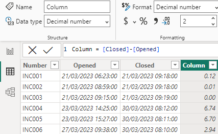
Let’s take a look with an example based on my scenario. This is my table:
I will create a new column to know the number of closing days:
I will create another one with the same formula but formatted as whole number so we can compare:
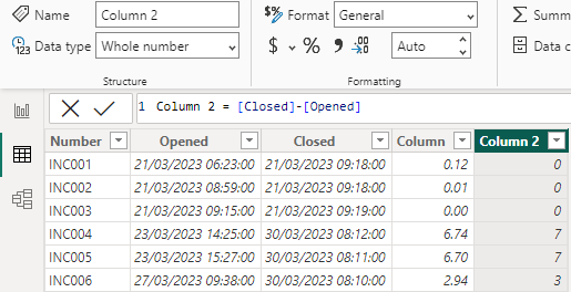
Remember I told you that putting it in whole number, it will round up or down:
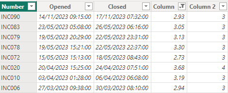
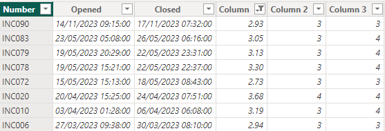
So selecting 3, I will have a range from 2.73 until 3.30 (normally it should be 2.5 until 3.5 but for my data, I don’t have those values). This is not what I want, I want by selecting 3, only the range from 2.73 until 3.00. I will create another column with my formula:
Now, we can see that numbers above 3.00, it is 4:
Interesting Management
-

Part 1: A good manager, better team motivation, better team productivity, better team results
When you are managing a team, “how to be a good manager” is the “must”...
-

Report optimization, increase your time management
As manager, I am doing many reports, even when I was an ITIL consultant, I still needed to do many reports...
-

Tools to get your ITIL intermediate certifications, the missing 15 points for the ITIL 4 Managing Professional
ITIL V3 is going to be obsolete...
-

The importance of the first customer meeting for the service
Managing an IT service when I start a new company is not an easy task, particularly true, if the service...
-

1 click macro tool: Incident/Problem Management - create a daily report in excel
This file will allow you to have in one single excel file the issues (incidents, problems, outages, major incidents...
-
1 click macro tool: Incident/Problem Management - create a daily report and a public version in excel
This file is an extended version of the above that includes the option to create a public version to share with...
-
1 click macro tool: Problem/Incident Management - compile multiple daily excel files in 1 with access
This file will allow you to compile all daily issues reported in excel in 1 single excel file in xlsx format...
-
1 click macro tool: Incident/Problem Management - create a monthly report in excel
This file will allow you to create a monthly report related to daily issues and updating all pivots, charts and...
-
1 click macro tool: Problem/Incident Management - create daily reports and compile them in 1 to create the monthly report in excel
This tool will create daily reports then compile them to create the monthly...
-

Calculate a weighted average for a SLA and a conversation time with a formula in an excel report
In one of my experiences, I had a tool that gave me the weighted average...
-
Search in different sheets then display the wanted data with a formula in an excel report
vlookup and hlookup are formulas that allow to search a data in another...
-
Find the good data by matching 3 different criterias with a formula in an excel report
It is a combination of “index” and “match” formulas, much better...
-
Sum and count sales with a formula in an excel report
Extracting data from salesforce or qlikview may not give the information I needed, it already happened...
-
Know how long a service is impacted with a formula in an excel report
It is important to know how long the service has been impacted by...